Introduction

We examine here the particularities of refining a model in a 2D context. As explained in a KB article on solving accuracy, it is sufficient to stabilize the quantity of interest with respect to the following six model settings:

1. The CG tolerance;
2. The Newton tolerance;
3. The air box size;
4. The time step;
5. The polynomial order (PO);
6. The mesh refinement.

The CG tolerance is quite irrelevant in 2D because the default solver technique is the direct method, which routinely resolves the matrix system within a tolerance much smaller than the default CG tolerance of 0.01%. The Newton tolerance remains relevant when the model has nonlinearities, but problems with the default Newton tolerance of 1% are not nearly as common as they tend to be in 3D solving. The air box size is relatively easy to guess and to optimize if necessary, while the time step is only relevant in Transient simulations and is also straightforward to optimize (although testing can be time-consuming).

For the above reasons, the work of refining a 2D model often boils down to the challenge of choosing the combination of PO and mesh refinement that will deliver the quantity of interest within the required accuracy level and using the smallest possible computing time. The user is often confused by the fact that increasing the model's PO (the only PO setting available in 2D) and increasing the mesh density have the same effect of increasing the number of degrees of freedom in the solution domain. For an equal number of degrees of freedom, however, a higher PO has the advantage that the field behavior is estimated using higher-order basis functions. This advantage is often left unexploited by users because the program interface seems designed to focus their attention on the mesh at the expense of the PO:

• The default PO for 2D Cartesian models is the lowest possible value of 1 (2 for 2D axisymmetric models);
• 2D mesh viewing shows the mesh nodes, which correspond to the degrees of freedom that pertain to a PO of 1. At higher POs, the degrees of freedom can be much more densely distributed than the mesh view suggests, and hence the mesh view can be severely misleading because it conveys the mesh's contribution to the number of degrees of freedom, but not the PO's contribution.

Another disadvantage of refining the mesh instead of raising the PO is that the meshing time itself will be increased and may easily overtake the total solving time. On the other hand, raising the PO alone is of limited potential benefit because one must stop at PO 4. Therefore the possibility of having to refine the mesh can never be dismissed from the outset. This opens up a number of possible scenarios that are well illustrated in the example below.

Example model

The attached 2D Cartesian test model POMEStest0.mn will be used as a demonstration of our suggested approach to 2D model refinement. A simple round coil of Solid type has an imposed current of 1 A rms, and the quantity of interest is the coil's Ohmic Loss. The model has no nonlinearities, the air box is assumed to be adequate, and the solver is Time-Harmonic (no time stepping), leaving the PO and mesh refinement to be optimized. The default 2D mesh is shown below.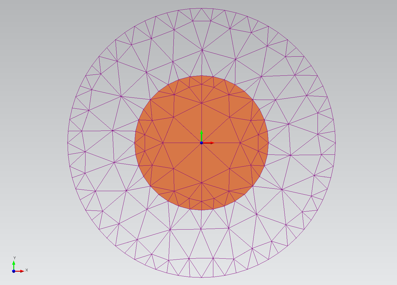

Optimization of the PO

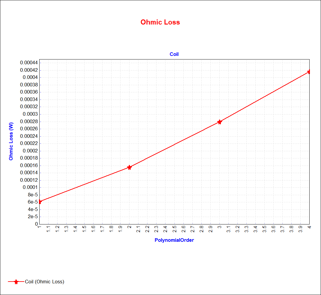
Four problems are defined for model POs of 1, 2, 3, and 4. For the starting Source Frequency of 100 kHz, the graph below shows the coil's Ohmic Loss as a function of Problem ID.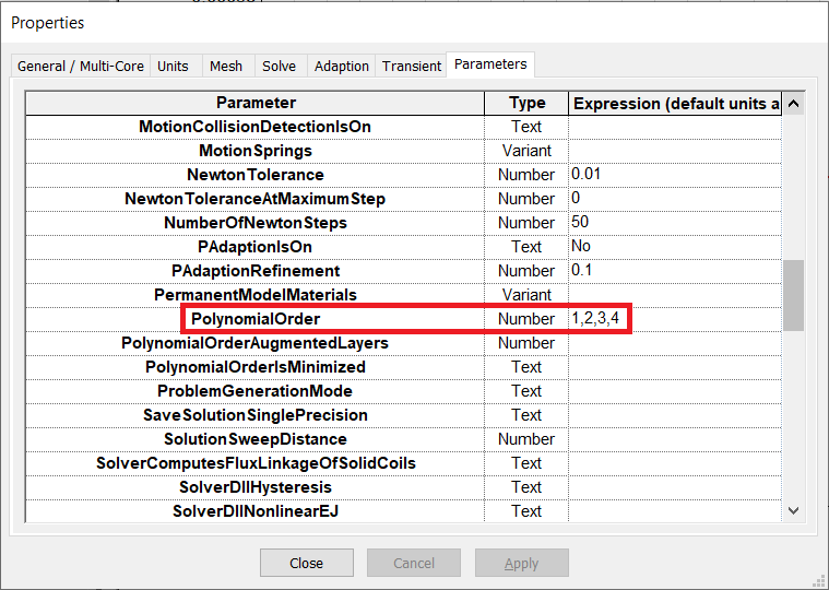

  

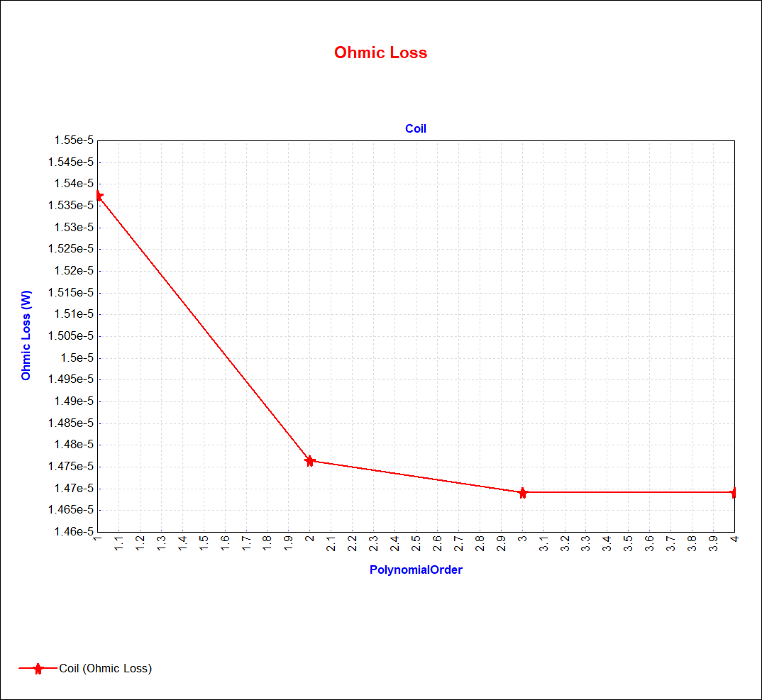
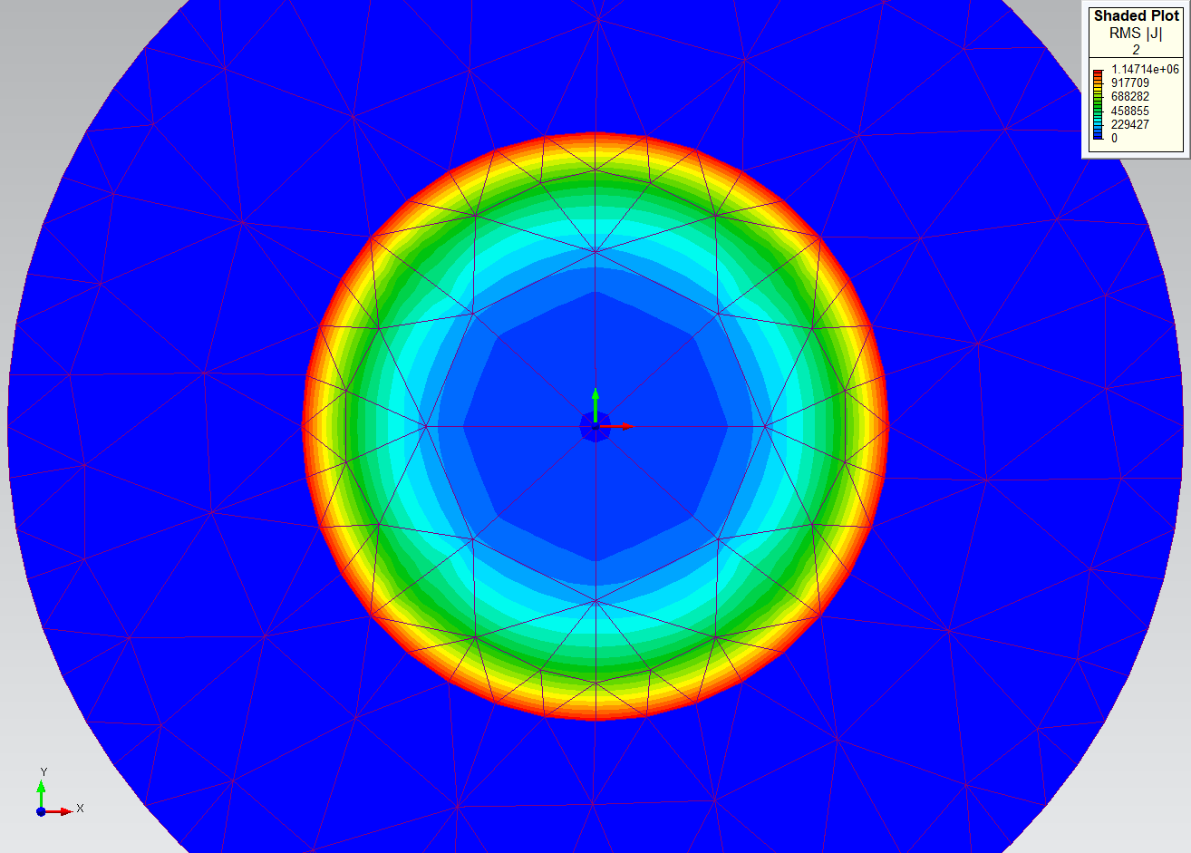
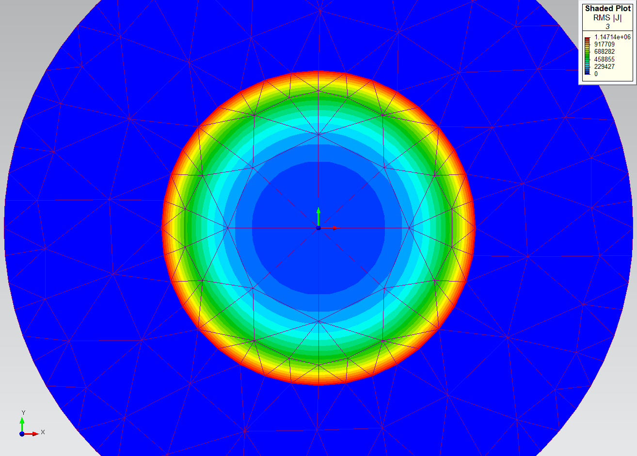
On this graph, the Ohmic Loss has stabilized at PO 3. Recourse to PO 4 is unnecessary, let alone further mesh refinement. For additional vindication, the shaded plots below show the progression of the RMS |J| field through PO 1, 2, and 3. It is important to note that if a PO of 1 or 2 is used instead of 3, further mesh refinement is able to raise the Ohmic Loss accuracy to the same high level observed at PO 3, but the resulting setup will take longer to solve than the PO 3 setup.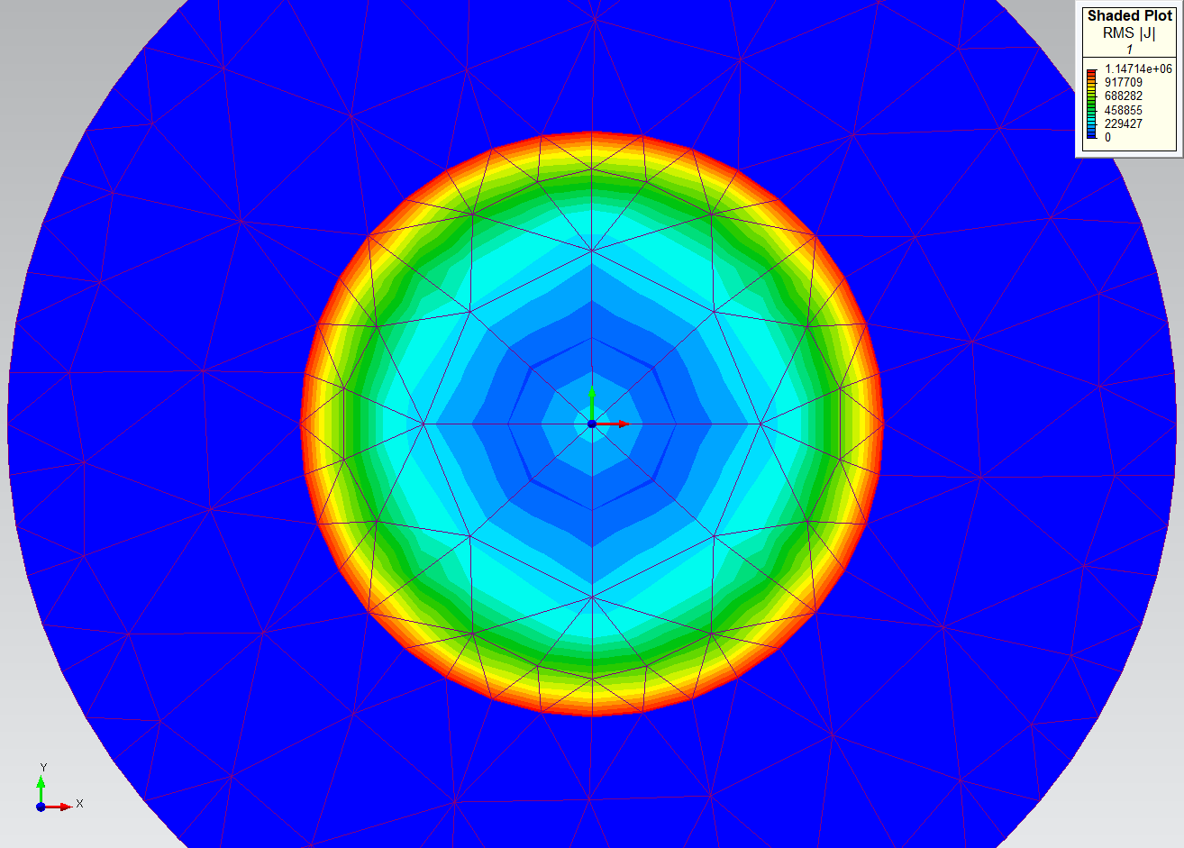

  



To raise the degree of difficulty, the Source Frequency is now raised by three orders of magnitude to 100 MHz, causing the skin depth to shrink by a factor of almost 32. After solving the four problems again, the graph of Ohmic Loss shows movement, but no final convergence.

The plots of RMS |J| for problems 1-4 are shown below. Using consistent upper and lower bounds in their color scales, the plots show that the higher order mesh elements are able to capture more of the current density in the shallow skin region.

  

  

At this point the model's polynomial order is set to the single value of 4, and means of further mesh refinement must be contemplated. There is much reason to refine the mesh strategically, given the highly localized skin effects. This can be accomplished automatically or manually.

Automatic mesh refinement

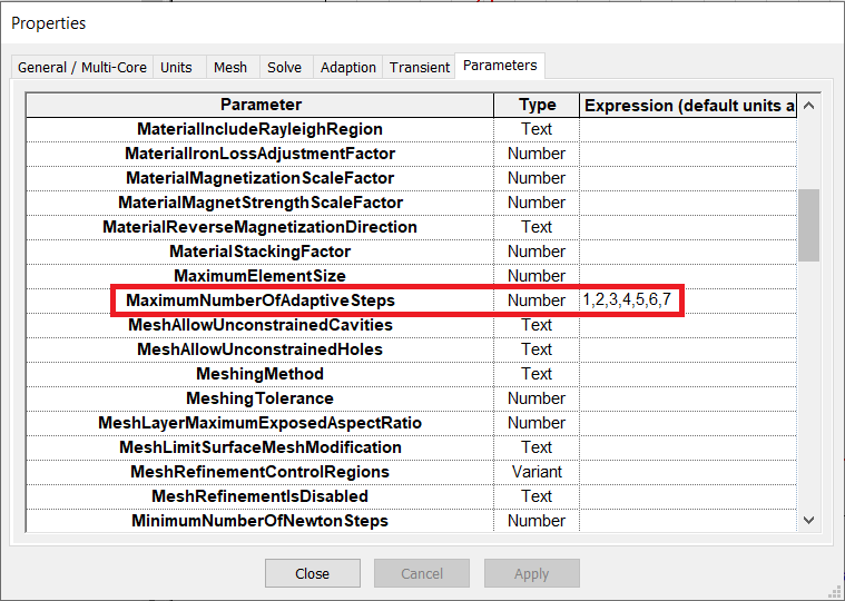
The figures below illustrate the gradual phasing in of the automatic method of strategic mesh refinement. In the Adaption Options dialog (left), h-adaption is turned on, and the number of adaption steps is forced to the maximum number via an impossibly low adaption tolerance. Then 7 problems are defined by setting MaximumNumberOfAdaptiveSteps to values between 1 and 7. Note that this parameter actually refers to the total number of solutions and therefore the number of adaption steps will range from zero (no adaption at all) to 6.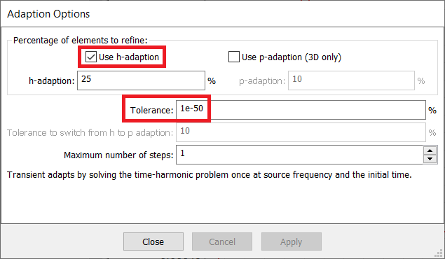

  

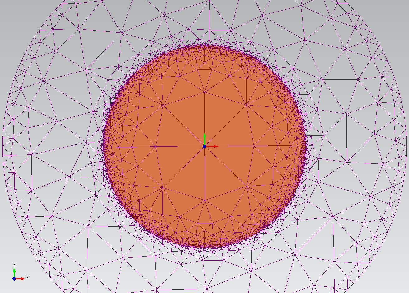
The left figure below shows the progression of the total Ohmic Loss through the 7 problems. The Ohmic Loss is well converged at Problem 5, i.e. after 4 steps of h-adaption. The right figure below shows the adapted Solution Mesh for Problem 5. As expected, the mesh refinement has focused on the surface of the coil.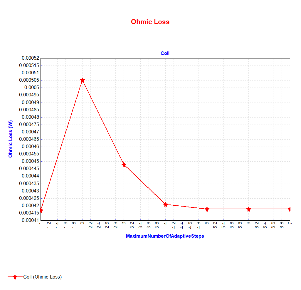

  

H-adaption may be helpful in detecting phenomena too localized to be noticed in a field plot, but the quality of its results can vary widely. It is not meant for efficiency, and its focus may not always be in the interest of the quantity being monitored.

Manual mesh refinement

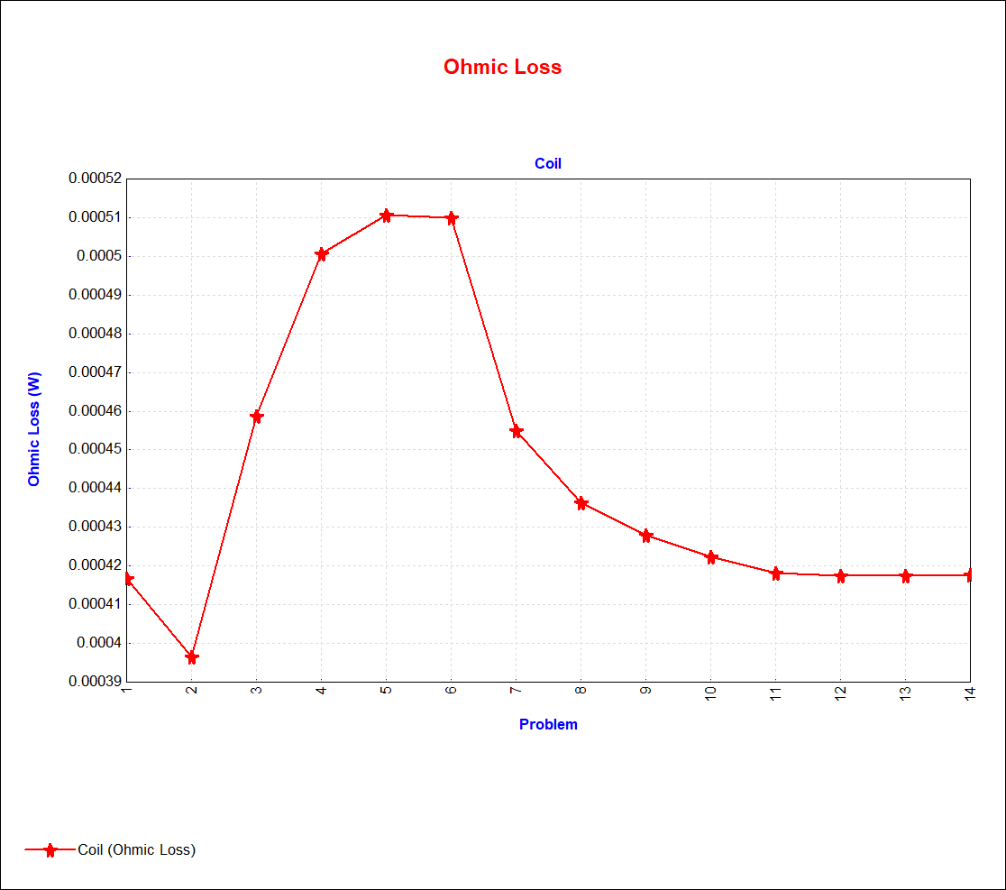
The more experienced user will use his knowledge of electromagnetics to manually refine the mesh in the areas of greater strategic importance to his quantity of interest. In the attached second test model POMEStest.mn, a Maximum Element Size (MES) is assigned to the two sides faces of the coil component. The MES is assigned 14 exponentially decreasing values, the first of which amounts to no change to the default mesh. The figures below show the Problem page and the progression of the Ohmic Loss through the 14 problems. The Ohmic Loss is well converged at Problem 12.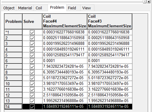

  

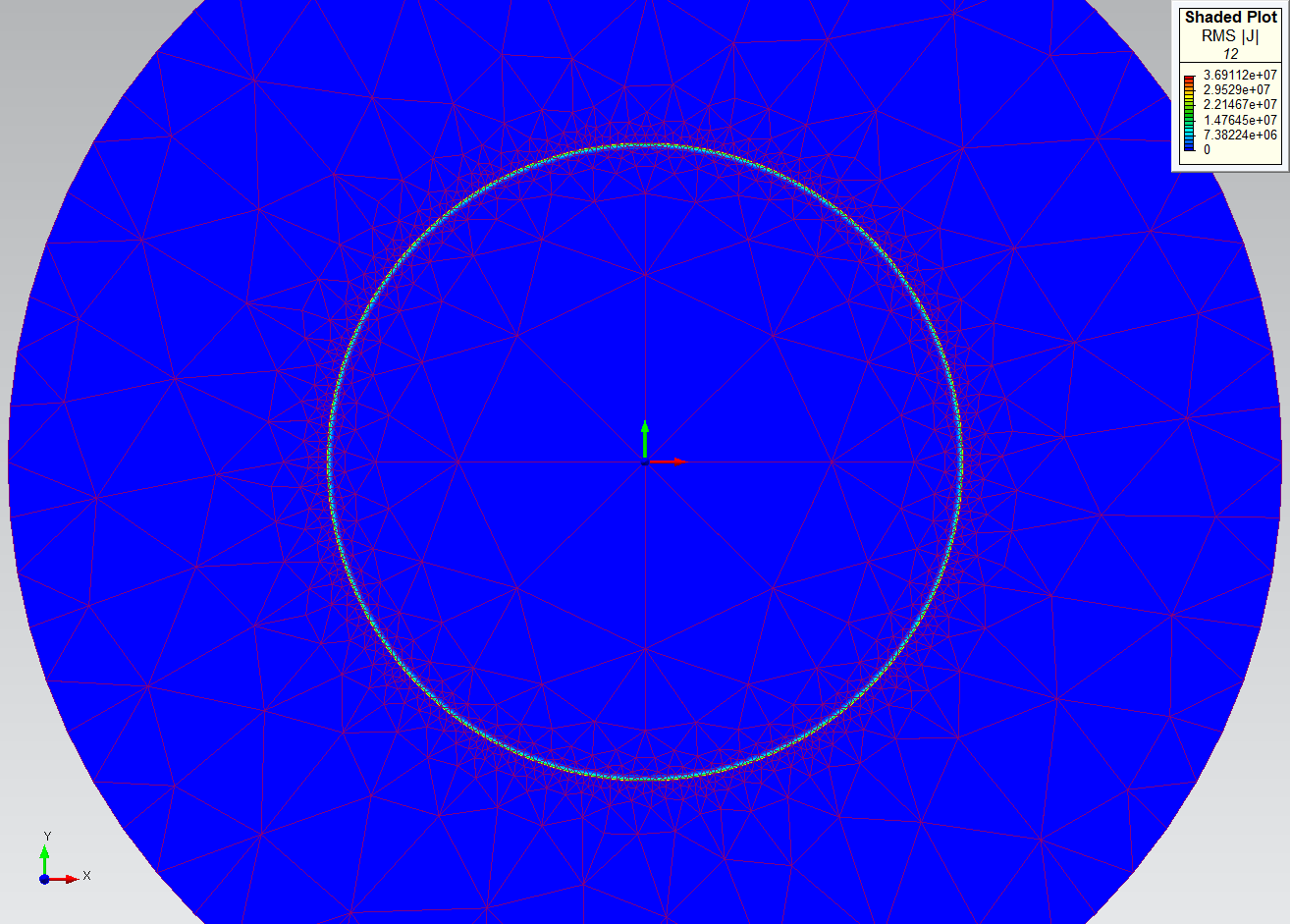
The RMS |J| field and the Solution Mesh at Problem 12 are superimposed in the plot below.