Simcenter Testing Solutions Overlap: What, Why and How to use it
2022-01-10T21:42:42.000-0500
Simcenter Testlab
Summary
Details
Overlap: What, Why and How to use it
Direct YouTube link: https://youtu.be/etrCZOY9Gtc
Introduction
Overlap is a parameter used when determining the way time data is to be processed and converted into the frequency domain. It can have a big effect on the results, so understanding overlap is critical to a successful data processing session. This article will explain what overlap is, why it is useful, and show how it is applied in Simcenter Testlab software.
This article contains the following sections:
1. What is “overlap”?
1a. Overlap definition:

When processing data, be it from a microphone, accelerometer, or any other device, to view the frequency content of the signal we need to take a block of the time data and send it through the Fast Fourier Transform or FFT. For the purposes of this article, we will refer to this block of time data as the “observation time,” and denote it using a capital T. Observation time (T) is measured in seconds and is the amount of time data used for one FFT calculation (Figure 1).
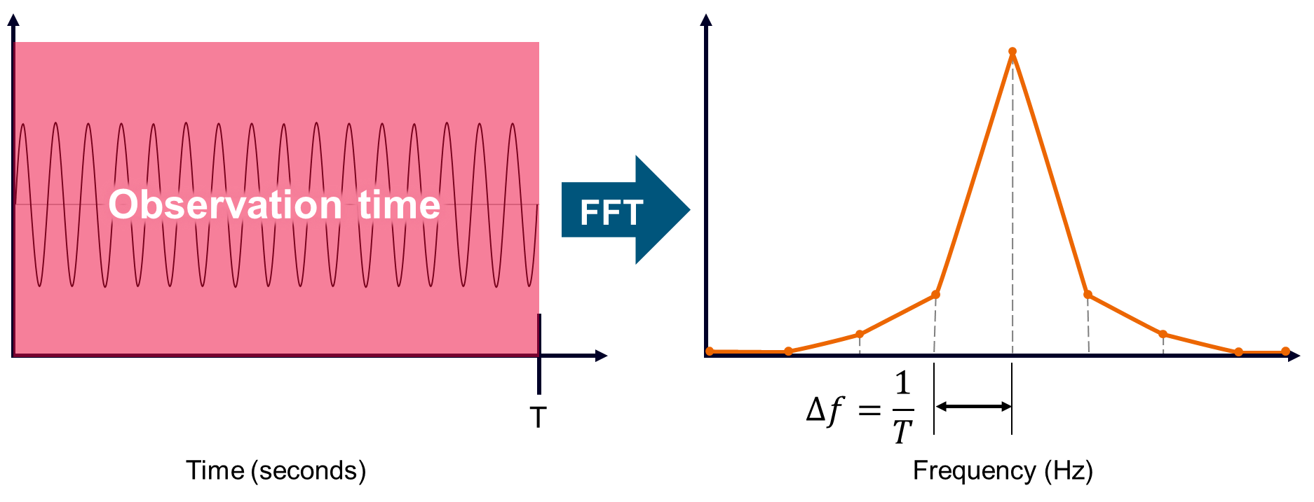
Figure 1. The observation time (T) is the amount of time data used for a single FFT.
As the name suggests, overlap occurs when two neighboring observation time blocks overlap each other and include the same time data. Overlap is designated as a percentage (%) and refers to the percentage of the observation time T that is overlapping the neighboring observation time block (see Figure 2).
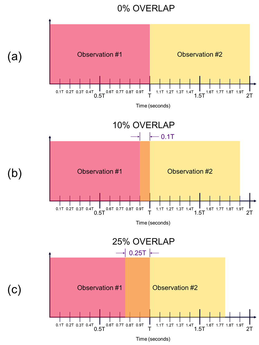
Figure 2. Overlap is specified as a percentage of the observation window time (T). Three values of overlap are shown: 0% Overlap (Figure 2a), 10% Overlap (Figure 2b), and 25% Overlap (Figure 2c).
The overlapping observations means the time data in the overlapped portion belongs to more than one FFT calculation. The overlapping observation times also result in less of the original time data being utilized for a fixed number of observations. For example, note in Figure 2a that two FFTs with 0% overlap uses a full 2T amount of time data, while in Figure 2c the same two FFTs overlapped 25% only uses 1.75T worth of time data.
So now that we know what overlap is, why is it useful? Two reasons will be covered in the next sections.
1b. Window effects
When investigating the frequency content of a measured signal, effectively using overlap can make the difference between getting the correct answer and completely missing important frequency content in your processed results (see Figure 3). The “dots” in the top plot of Figure 3 (0% Overlap) are caused by a window function used during the FFT calculation. Applying overlap can help overcome these window effects if used properly. The bottom plot of Figure 3 (90% Overlap) shows accurate amplitude levels for the orders (diagonal lines) across all frequencies and moments in time.
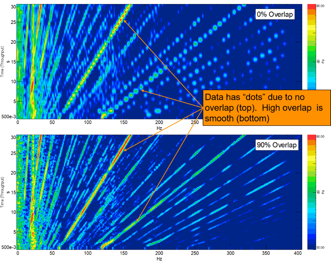 Figure 3. Effectively used overlap can overcome windowing effects applied during the FFT process and reveal additional frequency & amplitude information that otherwise may have been missed.
In order to reduce spectral leakage, oftentimes a window function is applied to the observation time block prior to the FFT operation. The most popular window function for typical noise and vibration data is called the Hanning window and is shown in Figure 4 below. Due to its popularity, the Hanning window will be the window used for demonstrations and examples throughout the duration of this article.
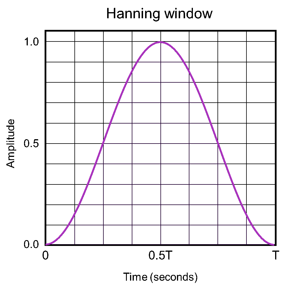
Figure 4. The Hanning window is a general-purpose window for reducing leakage in FFT calculations. The window is zero (0) at the beginning and end, with a value of 1.0 at the midpoint.
The Hanning window function gradually transitions from a value of zero at the beginning of the time block (0T) to a value of 1.0 at the midpoint (0.5T), and back to zero at the end (T). Multiplying the original measurement signal by this window function makes the signal periodic within the observation time (T) by forcing the function value to be zero (0) at the beginning and end of T. This results in a new, modified signal which differs from the original measurement (see Figure 5).
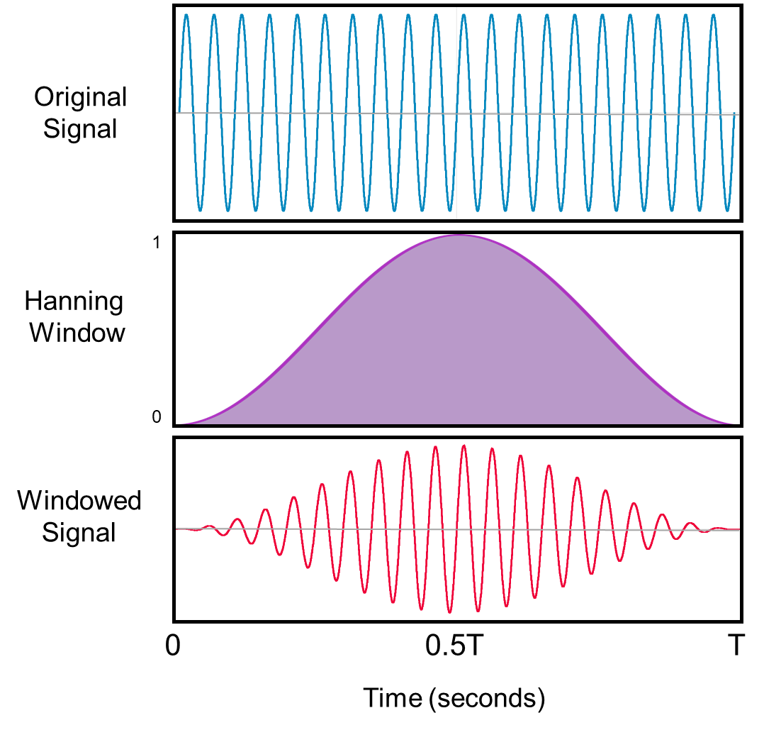
Figure 5. Original signal (top) is multiplied by a Hanning window (middle) to create a signal that has a value of zero at the beginning and end of the observation time T (bottom). This forces the windowed signal to be periodic within the observation time and reduces spectral leakage.
Supposing we want to make more than one FFT calculation over the course of our time data (as was done in Figure 3), we will need to consider the effect of the window functions used for each observation. If we process our time data with the observation times one after another with no overlap there will be portions of our original measurement that will not be used in any of the FFT calculations, as these portions are zeroed-out by the window (see Figure 6 below).
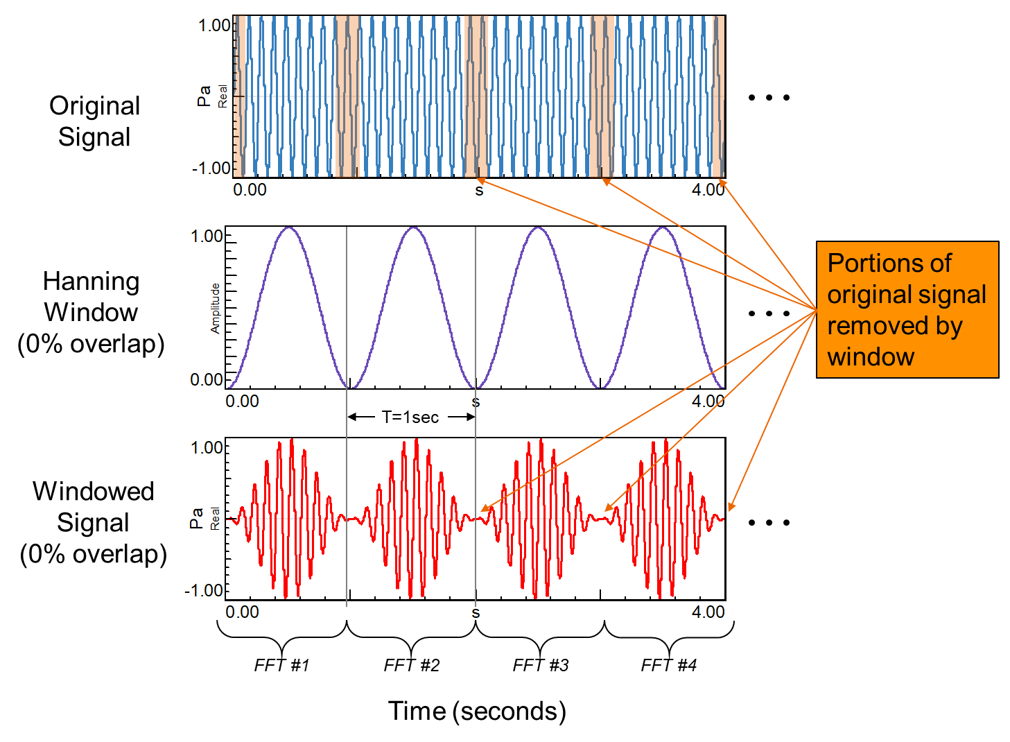
Figure 6. Original signal (top) is multiplied by a Hanning window (middle) to create a signal that has a value of zero at the beginning and end of the observation time T (bottom). As a result, portions of the original signal are removed from the FFT calculations.
Consider a recording of a sine wave (Figure 6, top). If we choose to set the observation time to 1 second (T=1.0 second) and apply a Hanning window with 0% overlap (Figure 6, middle), we will end up with a 1-second FFT calculation for each second of the recording (Figure 6, bottom). The Hanning window has forced our measured signal to be periodic within our observation time, but in doing so has removed part of the original signal. These portions removed by the window cannot be recovered and will not be included in any of the FFT calculations.
In order to reduce the amount of data loss due to windowing, the observation times (and accompanying windows) can be overlapped. In the specific case of the Hanning window, the optimal minimum overlap is 50% - such that the maximum of the neighboring Hanning window is centered on the end of the previous observation block, where the Hanning window is at its minimum (see Figure 7). The 50% overlapped Hanning windows work together to ensure all parts of the original time signal will be processed, and nothing will be completely omitted. This effect is shown in Figure 8 below.
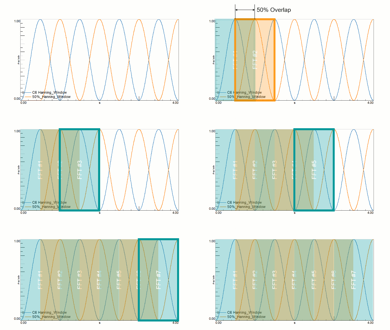
Figure 7. Overlapping Hanning windows at 50% aligns the maxima and minima of neighboring windows so all of the original measurement signal is captured in the FFT calculations.
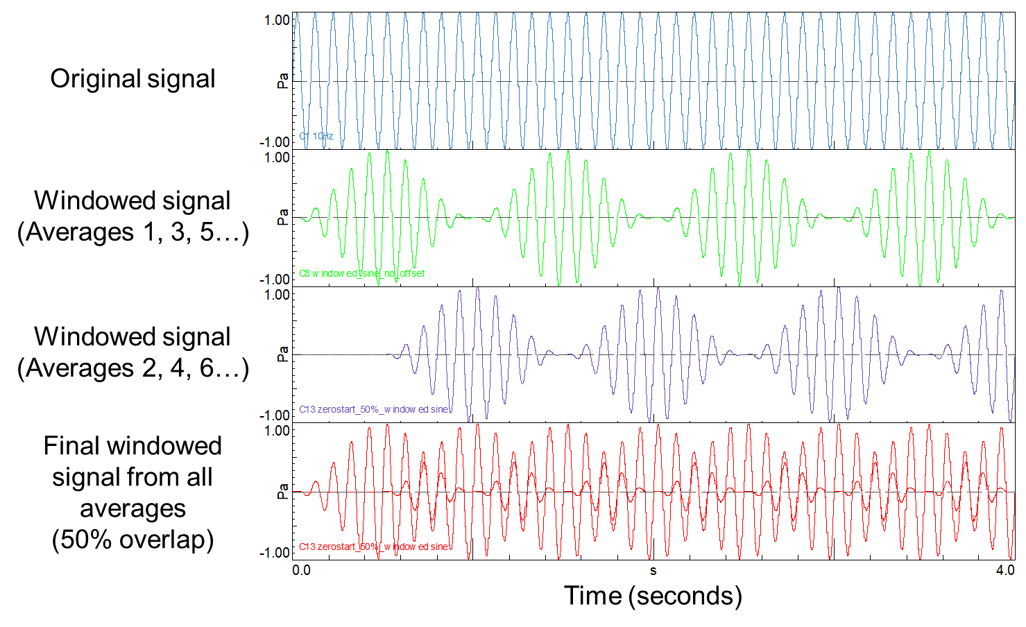
Figure 8. Hanning windows overlapped at 50% offset the zeroing effects of the individual windows, and results in nearly all data from the original signal being included in the FFT calculations.
1c. Data insights
When processing data versus time or other tracking parameter, overlap can be used to improve the usefulness of processed results. Depending on how it is applied, overlap can help in two ways: either by providing additional detail on how a quantity is changing over time, or by providing a smoothing effect, making trends in the data more obvious (see Figure 9).
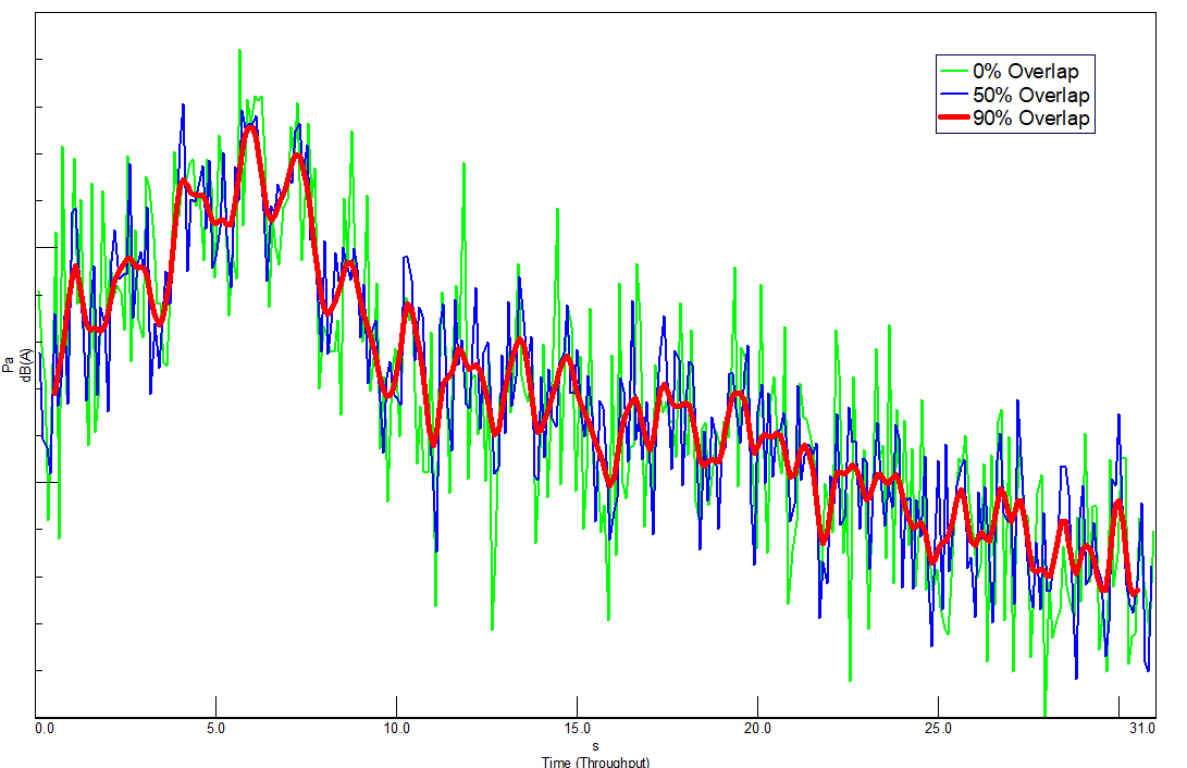
Figure 9. Increasing overlap can provide a smoothing effect and help make trends in data easier to observe. The fluctuating amplitude (green, no overlap) makes the trend in amplitude appear complicated. By increasing the overlap (red, 90% overlap) the trend of the amplitude is simplified and easier to interpret.
It has already been shown that increasing overlap results in more calculations per unit time. This effect can be used to gain additional granularity on how a quantity in the data is changing with respect to time by increasing the number of calculations in a given measurement length.
Conversely, in an instance where the data contains amplitude fluctuations which may be obfuscating an important trend, increased overlap can help to smooth these fluctuations, and make the trend easier to discern, as shown in Figure 9. These two overlap effects will be demonstrated on some examples in Section 3.
2. Simcenter Testlab Stationary Averaging and Overlap
2a. What is stationary averaging?
When multiple observation time blocks are processed for a given measurement (Figure 10a), one can specify how the FFT of these blocks are visualized in the frequency domain. In stationary averaging, the FFTs of observation time blocks #1 to #N are averaged together to produce a single frequency spectrum (Figure 2b). The other option is called tracked processing (Figure 10c) and will be discussed in section 3.

Figure 10: A time varying signal can be converted to the frequency domain using multiple observation time blocks (Figure 10a). The FFT of these time blocks can be averaged together to produce a single averaged spectrum (Figure 10b). This is known in Simcenter Testlab as stationary averaging.
Overlap plays a vital role in stationary averaging and can make the difference between calculating the correct answer and completely missing important frequency content!
2b. How is overlap specified?
In Simcenter Testlab the type of processing (stationary vs tracked) is selected in the Acquisition parameters dialog of Throughput Processing. The selection is made in the Measurement mode dropdown as shown in Figure 11 below.
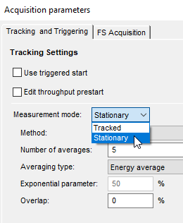
Figure 11. Measurement mode determines tracked or stationary processing.
Once Stationary averaging is selected, the user can then select the Method. Options are Free Run, Time and Event. The Event method allows the user to calculate averages only when certain other criteria are met by the data (like a trigger function) and will not be discussed here.
The most straight-forward method to calculate an averaged spectrum with a particular amount of overlap is to choose the Free Run method, as shown in Figure 12.
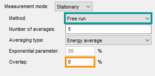
Figure 12. Free Run method allows for the overlap percentage to be explicitly set by the user.
With Free Run, the user specifies how many averages to take, and can specify the overlap percentage directly, regardless of any other parameters such as observation time (called “frame size” in Throughput processing). Averages will be computed until the number of requested averages have been calculated, or the end of the time history is reached. So, by setting the number of averages to a large value (i.e. – 5000) a user can ensure that averaging will continue at the specified overlap for the entirety of the measurement.
Obviously, the observation time (frame size) will also play a part in the number of averages calculated for a given time history, but the Free Run method automatically adjusts the number of averages per second to maintain the correct amount of overlap, whether the frame size is 1 second (1 Hz resolution) or 10 seconds (0.1 Hz resolution).
With the Time method, the situation is a bit reversed. Here, the user specifies the number of averages per second, regardless of frame size or overlap percentage (Figure 13).
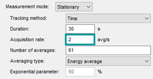
Figure 13. Time method of stationary averaging allows the user to specify a number of averages per second. Overlap will be a function of this number, as well as the frame size selected.
So, for a given Acquisition rate (averages per second), the amount of overlap will be a function of the specified frame size (or frequency resolution). The frame size and corresponding frequency resolution are set on the “FS Acquisition“ tab of the Acquisition parameters dialogue as shown in Figure 14 (red box).
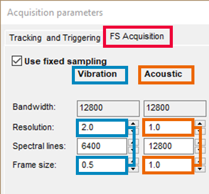
Figure 14. When using the Time method in stationary averaging, the frame size must be taken into account, as it will work in tandem with the acquisition rate to determine the resulting overlap percentage.
With the Time method in stationary averaging, the amount of overlap used in the averaging will be a function of the acquisition rate (averages per second) and the frame size (inverse of the frequency resolution).
As an example, consider the values specified in Figures 13 & 14. The acquisition rate is set to 2 averages per second (teal box, Fig 13). This means every 0.5 seconds we will initiate a new observation frame, or average, regardless of how long the observation frame is. If we consider the frame sizes shown in Figure 14, we see the channels in the Vibration group (blue boxes, Fig 14) have a frame size of 0.5 seconds (2 Hz resolution), while the channels in the Acoustic group (orange boxes Fig 14) have a frame size of 1.0 second (1 Hz resolution). So, every 0.5 seconds we are initiating an observation frame of 0.5 seconds for the channels in the Vibration group, and every 0.5 seconds initiating an observation frame of 1.0 second for the Acoustic group channels (see Figure 15).
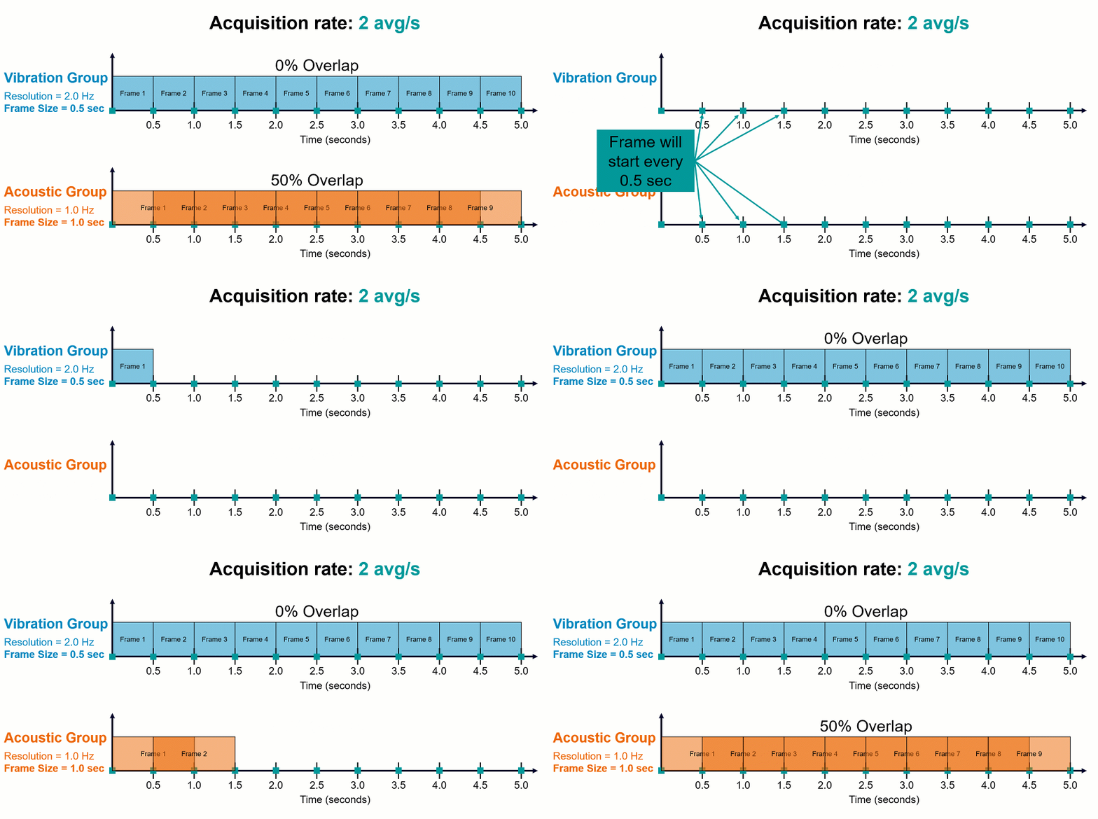
Figure 15. Acquisition rate and frame size work together to determine the overlap when using the Time method of tracking. Both groups are processed with the same acquisition rate of 2 averages/sec. The difference in frequency resolution (Vibration=2 Hz, Top. Acoustic=1 Hz, Bottom) results in different percentages of overlap being used for the two groups.
This means that the averaged spectra for the Vibration group will be calculated with 0% overlap, while the averaged spectra for the Acoustic group will be calculated with 50% overlap. If a specific amount of overlap is desired, both the acquisition rate (averages per second) and the frame size must be taken into account when using the Time method to calculate an averaged frequency spectrum.
2c. Example: Stationary averaging
To illustrate the benefit of using overlap during stationary averaging, consider the signal shown in Figure 16. The measured signal is primarily a sinusoid, but with occasional high-frequency transient events. The end goal is to investigate the signal’s frequency content by calculating an averaged frequency spectrum using stationary averaging in Simcenter Testlab.
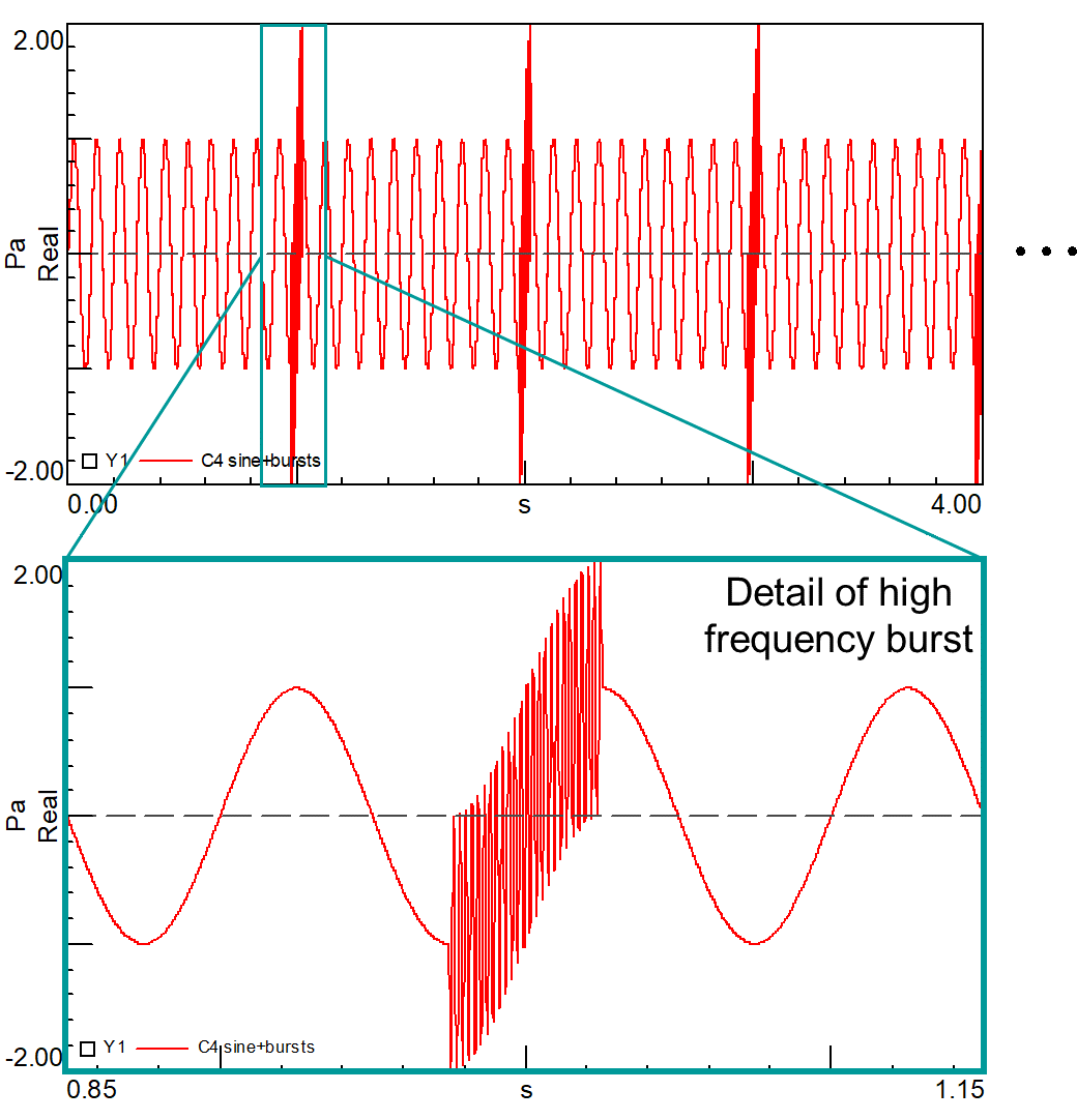
Figure 16. Top: Original signal; Sine wave with occasional bursts of higher frequency content. Bottom: detailed view of transient burst.
First, consider processing the measured signal with no overlap, and again using a 1-second observation time. This sets up the windowing scenario shown in Figure 17 below. Due to there being no overlap between the observation times, the Hanning windows completely remove the additional burst portion of the signal. As a result, this spectral content will be missing from the resulting frequency spectrum!
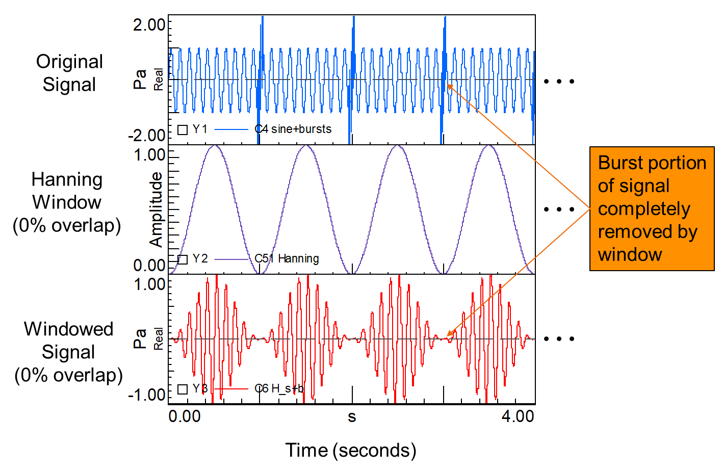
Figure 17. Original signal (top) is a sine wave with occasional bursts of higher frequency. A 1 second Hanning window is applied with no overlap (middle), resulting in the windowed signal (bottom). The windowed signal does not capture all the content of the original signal.
To minimize the impact of the Hanning windows on the processing of the original signal, an overlap of 50% is specified (Figure 18). With an observation time T = 1 second, 50% overlap means the second FFT calculation will begin half a second into the first observation time: odd-numbered observations begin on the integer values of time (0 s, 1 s, 2 s, etc) and the even-numbered observations begin on the half-second marks of the measurement (0.5 s, 1.5 s, 2.5 s, etc).
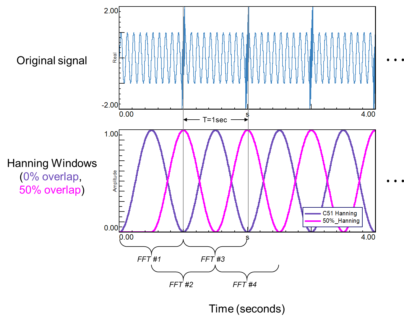
Figure 18. Hanning windows overlapped at 50% offset the zeroing effects of the individual windows.
The odd-numbered observations will capture the sinusoid portion of the signal, and the even-numbered observations will be centered on the burst portion of the signal. The resulting reconstructed signal from all observations (even and odd numbered) will include nearly all the original signal content (Figure 19). Notice overlapping the observation times will also result in more calculations per unit time compared to no overlap.
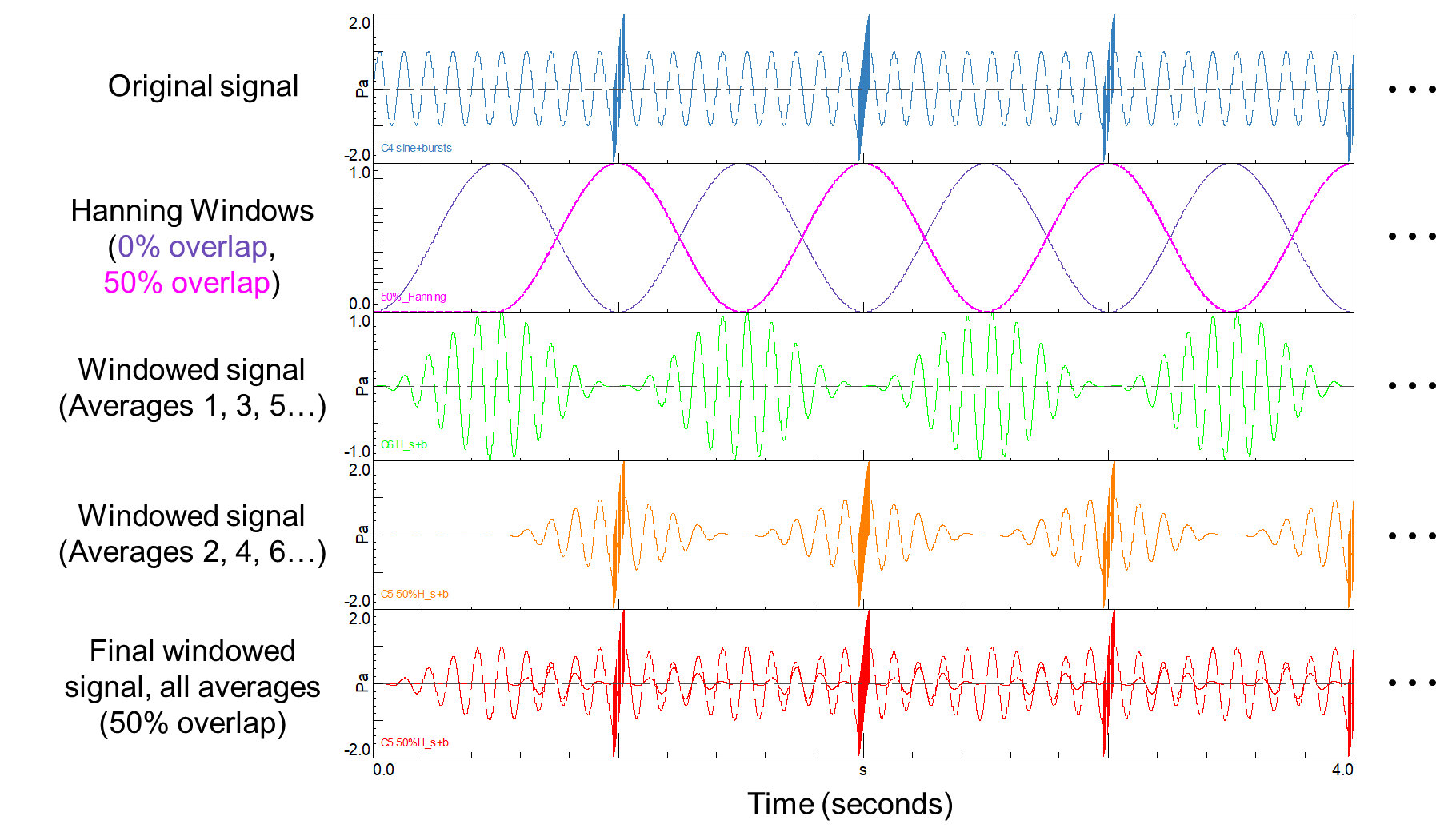
Figure 19. Hanning windows overlapped at 50% offset the zeroing effects of the individual windows, and result in nearly all data from the original signal being included in the FFT calculations.
The resulting effect of overlap can be seen in the averaged frequency spectra of both processing sets (Figure 20). By including an overlap of 50%, the high frequency component of the original signal is discovered, while in the 0% overlap case this high frequency component of the signal was removed by the Hanning window. As a result of applying a Hanning window without any overlap during our processing, the frequency content of the burst does not appear in the averaged frequency spectrum!
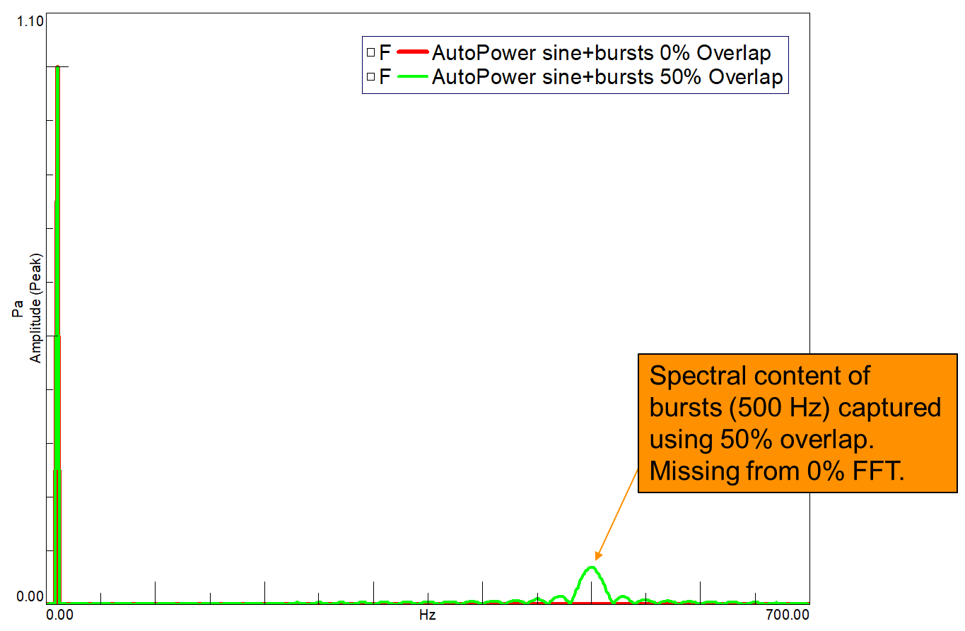
Figure 20. Averaged frequency spectra for both 0% overlap (red) and 50% overlap (green) time signals. Only the spectrum calculated using 50% overlap captures the frequency content of the periodic bursts. This content is removed by the windows when using 0% overlap.
3. Simcenter Testlab Tracked Processing and Overlap
3a. What is tracked processing?
Instead of combining and averaging the results of calculations like in stationary averaging, the results In tracked processing are kept separate and plotted against time, rpm, or other tracking parameter. This technique makes it possible to see how the calculation result changes as a function of the tracking parameter. Tracked processing is often used to plot multiple FFTs versus time or rpm, and plotted in a waterfall plot, or colormap (Figure 21c). It is also possible to calculate single number metrics, such as overall level (OAL), psychoacoustic loudness, RMS, etc, versus the tracking parameter to investigate how the quantity changes as a function of the tracking parameter.
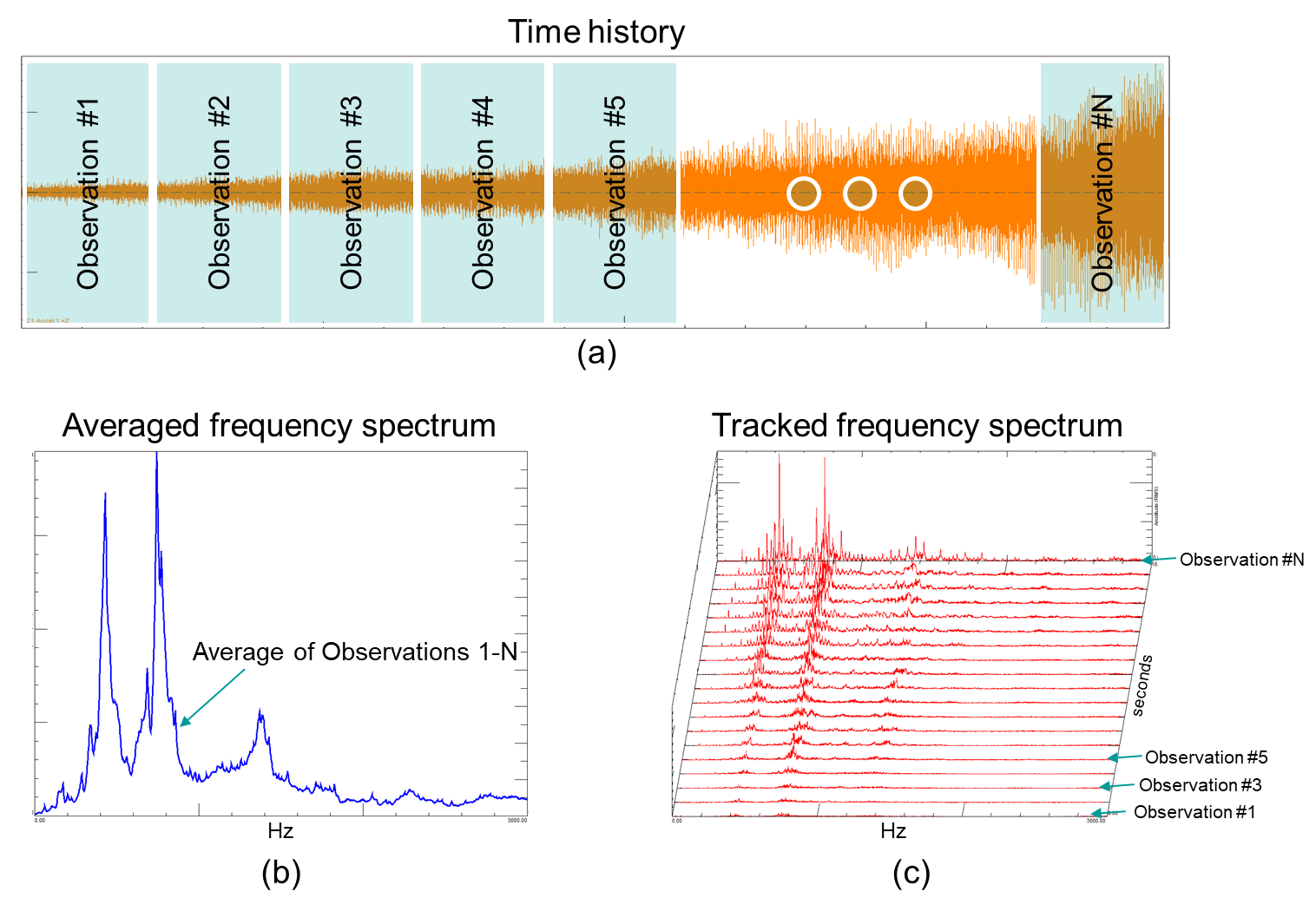
Figure 21: A time varying signal can be converted to the frequency domain using multiple observation time blocks (Figure 21a). The individual FFTs of these time blocks can be plotted in a 3-dimensional waterfall plot, with an axis for a tracking parameter (time, rpm, etc) (Figure 21b). This is known in Simcenter Testlab as tracked processing.
3b. How is overlap specified in tracked processing?
In Simcenter Testlab the type of processing (stationary vs tracked) is selected in the Acquisition parameters dialog of Throughput Processing. The selection is made in the Measurement mode dropdown as shown in Figure 22 below.
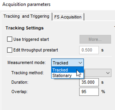
Figure 22. Measurement mode determines tracked or stationary processing.
Once Tracked processing is selected, the user can then select the Tracking method. Options are Free Run, Tacho, Time, Static and Event. The Tacho method is discussed in detail in this article and will not be covered here. Event allows the user to calculate averages only when certain other criteria are met by the data (like a trigger function) and Static allows to track on a static channel, such as temperature. These options are less frequently used and will not be discussed here.
As in Stationary averaging, the easiest way to perform tracked processing with a specific overlap percentage is to select the Free run mode, which allows the user to specify the overlap directly in the interface, as shown in Figure 23 below.
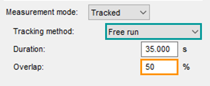
Figure 23. Free run tracking method allows the user to specify overlap percentage directly.
Here the user specifies the duration of the processing, rather than a number of averages like in Stationary averaging. To ensure the entire time history is processed, the Duration entered should be at least as long as the measurement. Enter the Overlap % and Testlab will automatically adjust the calculation increment based on the frame size to ensure the proper overlap.
Using the Time method in tracked processing is very similar to how it is used in stationary averaging. In tracked processing, the user specifies an increment, which is the amount of time between calculations. If this is set to 0.5 seconds as shown in Figure 24 below, an observation frame will be initiated every 0.5 seconds, regardless of how long the frame is. Similar to stationary averaging, the amount of overlap in tracked processing will be a function of both the increment and the frame size when using the Time tracking method.
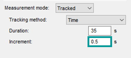
Figure 24. In the Time tracking method, the user specifies the increment (time between observations), and overlap will be a function of increment and frame size.
3c. Tracked processing examples
When calculating a metric versus time for a measurement (i.e.- overall level, RMS, loudness, etc), overlap can be included in the processing, just as it is when performing stationary averaging. In tracked processing, there are two primary options or techniques to specify a particular amount of overlap in Simcenter Testlab: Free-run and Time. However, the two techniques have opposite effects on the resulting data. These effects are covered in the following examples.
3c.1 Using overlap to increase the number of data points
Free Run: In free run, the amount of overlap is specified directly by the user. Increasing the overlap percentage will result in an increased number of calculations for the record length. This increase brings some additional insight into the time-variation of the calculated metric: the more data points calculated for a given record length means more specificity with respect to time. This effect is shown below in Figure 25.
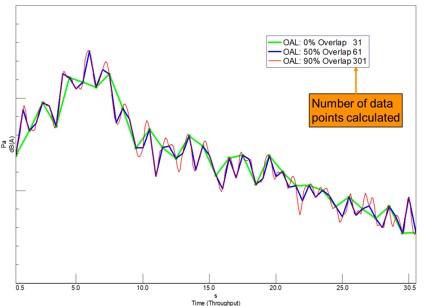
Figure 25. Effect of increased overlap on overall level versus time calculations. Increasing overlap results in more data points, which brings more detail to the overall level variation versus time (red). With no overlap, fewer data points are calculated, resulting in less detail versus time (green).
Overall level was calculated with different amounts of overlap: 0%, 50%, and 90%. Increasing the amount of overlap results in more values being calculated, as shown in the legend of Figure 25. With no overlap (green) the overall level vs. time function has 31 data points. Overlapping at 50% (blue) results in 61 data points for the same record length. The amount of data points increases to 301 at 90% overlap (red). Notice the values of the three traces are identical when they intersect. Increasing the overlap allows for more insight as to how the overall level is fluctuating versus time.
3c.2 Using overlap to smooth amplitude fluctuation
Time: When selecting to track on time, the user specifies a fixed calculation increment. As a result, the processed data will all have roughly the same number of data points, regardless of the amount of overlap. However, because the time increment between calculations is fixed, the user must change the frame size, or observation time, for each calculation to change the amount of overlap. Increasing overlap means using a longer frame, which will result in a finer frequency resolution for FFT calculations and adds a smoothing effect to the trend of calculated values (see Figure 26).
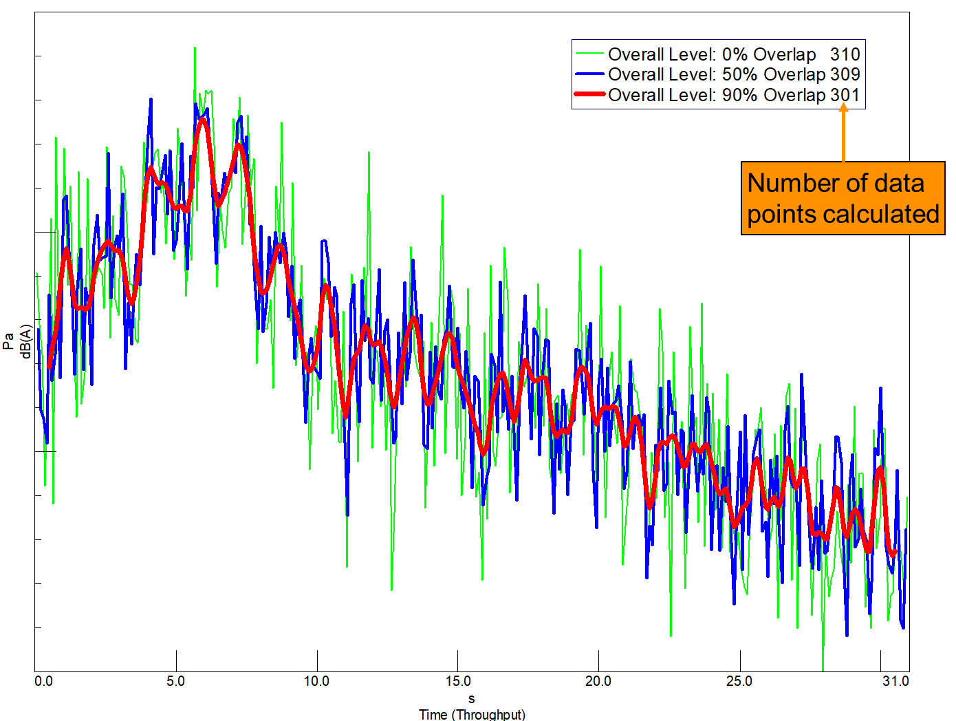
Figure 26. Effect of increasing overlap with a constant increment. The longer frame size needed to create the overlap has a smoothing effect (red) on the amplitude variation, while maintaining roughly the same number of data points. With no overlap, the amplitude variation is much greater (green).
Increasing the overlap averages more data points together for each increment step, which simplifies the trend and removes amplitude jitter. In this case, the increment was set to 0.1 seconds to preserve the detail of the changes in overall level versus time. The 0% overlap trace (green) features a frame of 0.1 seconds, and has amplitude values that vary widely from point to point. For 50% overlap (blue) the frame is increased to 0.2 seconds, or twice as many data points being averaged together for each calculation. For 90% overlap (red), a full second is required for each calculation which results in a much smoother transition between data points. Note that all the traces in Figure 26 have roughly the same number of data points (approximately 300).
Questions? Email macdonald@siemens.com or simply comment on this article.
Related Links:
Direct YouTube link: https://youtu.be/etrCZOY9Gtc
Introduction
Overlap is a parameter used when determining the way time data is to be processed and converted into the frequency domain. It can have a big effect on the results, so understanding overlap is critical to a successful data processing session. This article will explain what overlap is, why it is useful, and show how it is applied in Simcenter Testlab software.
This article contains the following sections:
- What is overlap?
- Overlap definition
- Why: Window effects
- Why: Data insights
- Simcenter Testlab Stationary Averaging and Overlap
- What is stationary averaging?
- How is overlap specified?
- Examples
- Simcenter Testlab Tracked Averaging and Overlap
- What is tracked averaging?
- How is overlap specified?
- Examples
1. What is “overlap”?
1a. Overlap definition:
When processing data, be it from a microphone, accelerometer, or any other device, to view the frequency content of the signal we need to take a block of the time data and send it through the Fast Fourier Transform or FFT. For the purposes of this article, we will refer to this block of time data as the “observation time,” and denote it using a capital T. Observation time (T) is measured in seconds and is the amount of time data used for one FFT calculation (Figure 1).
Figure 1. The observation time (T) is the amount of time data used for a single FFT.
As the name suggests, overlap occurs when two neighboring observation time blocks overlap each other and include the same time data. Overlap is designated as a percentage (%) and refers to the percentage of the observation time T that is overlapping the neighboring observation time block (see Figure 2).
Figure 2. Overlap is specified as a percentage of the observation window time (T). Three values of overlap are shown: 0% Overlap (Figure 2a), 10% Overlap (Figure 2b), and 25% Overlap (Figure 2c).
The overlapping observations means the time data in the overlapped portion belongs to more than one FFT calculation. The overlapping observation times also result in less of the original time data being utilized for a fixed number of observations. For example, note in Figure 2a that two FFTs with 0% overlap uses a full 2T amount of time data, while in Figure 2c the same two FFTs overlapped 25% only uses 1.75T worth of time data.
So now that we know what overlap is, why is it useful? Two reasons will be covered in the next sections.
1b. Window effects
When investigating the frequency content of a measured signal, effectively using overlap can make the difference between getting the correct answer and completely missing important frequency content in your processed results (see Figure 3). The “dots” in the top plot of Figure 3 (0% Overlap) are caused by a window function used during the FFT calculation. Applying overlap can help overcome these window effects if used properly. The bottom plot of Figure 3 (90% Overlap) shows accurate amplitude levels for the orders (diagonal lines) across all frequencies and moments in time.
In order to reduce spectral leakage, oftentimes a window function is applied to the observation time block prior to the FFT operation. The most popular window function for typical noise and vibration data is called the Hanning window and is shown in Figure 4 below. Due to its popularity, the Hanning window will be the window used for demonstrations and examples throughout the duration of this article.
Figure 4. The Hanning window is a general-purpose window for reducing leakage in FFT calculations. The window is zero (0) at the beginning and end, with a value of 1.0 at the midpoint.
The Hanning window function gradually transitions from a value of zero at the beginning of the time block (0T) to a value of 1.0 at the midpoint (0.5T), and back to zero at the end (T). Multiplying the original measurement signal by this window function makes the signal periodic within the observation time (T) by forcing the function value to be zero (0) at the beginning and end of T. This results in a new, modified signal which differs from the original measurement (see Figure 5).
Figure 5. Original signal (top) is multiplied by a Hanning window (middle) to create a signal that has a value of zero at the beginning and end of the observation time T (bottom). This forces the windowed signal to be periodic within the observation time and reduces spectral leakage.
Supposing we want to make more than one FFT calculation over the course of our time data (as was done in Figure 3), we will need to consider the effect of the window functions used for each observation. If we process our time data with the observation times one after another with no overlap there will be portions of our original measurement that will not be used in any of the FFT calculations, as these portions are zeroed-out by the window (see Figure 6 below).
Figure 6. Original signal (top) is multiplied by a Hanning window (middle) to create a signal that has a value of zero at the beginning and end of the observation time T (bottom). As a result, portions of the original signal are removed from the FFT calculations.
Consider a recording of a sine wave (Figure 6, top). If we choose to set the observation time to 1 second (T=1.0 second) and apply a Hanning window with 0% overlap (Figure 6, middle), we will end up with a 1-second FFT calculation for each second of the recording (Figure 6, bottom). The Hanning window has forced our measured signal to be periodic within our observation time, but in doing so has removed part of the original signal. These portions removed by the window cannot be recovered and will not be included in any of the FFT calculations.
In order to reduce the amount of data loss due to windowing, the observation times (and accompanying windows) can be overlapped. In the specific case of the Hanning window, the optimal minimum overlap is 50% - such that the maximum of the neighboring Hanning window is centered on the end of the previous observation block, where the Hanning window is at its minimum (see Figure 7). The 50% overlapped Hanning windows work together to ensure all parts of the original time signal will be processed, and nothing will be completely omitted. This effect is shown in Figure 8 below.
Figure 7. Overlapping Hanning windows at 50% aligns the maxima and minima of neighboring windows so all of the original measurement signal is captured in the FFT calculations.
Figure 8. Hanning windows overlapped at 50% offset the zeroing effects of the individual windows, and results in nearly all data from the original signal being included in the FFT calculations.
1c. Data insights
When processing data versus time or other tracking parameter, overlap can be used to improve the usefulness of processed results. Depending on how it is applied, overlap can help in two ways: either by providing additional detail on how a quantity is changing over time, or by providing a smoothing effect, making trends in the data more obvious (see Figure 9).
Figure 9. Increasing overlap can provide a smoothing effect and help make trends in data easier to observe. The fluctuating amplitude (green, no overlap) makes the trend in amplitude appear complicated. By increasing the overlap (red, 90% overlap) the trend of the amplitude is simplified and easier to interpret.
It has already been shown that increasing overlap results in more calculations per unit time. This effect can be used to gain additional granularity on how a quantity in the data is changing with respect to time by increasing the number of calculations in a given measurement length.
Conversely, in an instance where the data contains amplitude fluctuations which may be obfuscating an important trend, increased overlap can help to smooth these fluctuations, and make the trend easier to discern, as shown in Figure 9. These two overlap effects will be demonstrated on some examples in Section 3.
2. Simcenter Testlab Stationary Averaging and Overlap
2a. What is stationary averaging?
When multiple observation time blocks are processed for a given measurement (Figure 10a), one can specify how the FFT of these blocks are visualized in the frequency domain. In stationary averaging, the FFTs of observation time blocks #1 to #N are averaged together to produce a single frequency spectrum (Figure 2b). The other option is called tracked processing (Figure 10c) and will be discussed in section 3.
Figure 10: A time varying signal can be converted to the frequency domain using multiple observation time blocks (Figure 10a). The FFT of these time blocks can be averaged together to produce a single averaged spectrum (Figure 10b). This is known in Simcenter Testlab as stationary averaging.
Overlap plays a vital role in stationary averaging and can make the difference between calculating the correct answer and completely missing important frequency content!
2b. How is overlap specified?
In Simcenter Testlab the type of processing (stationary vs tracked) is selected in the Acquisition parameters dialog of Throughput Processing. The selection is made in the Measurement mode dropdown as shown in Figure 11 below.
Figure 11. Measurement mode determines tracked or stationary processing.
Once Stationary averaging is selected, the user can then select the Method. Options are Free Run, Time and Event. The Event method allows the user to calculate averages only when certain other criteria are met by the data (like a trigger function) and will not be discussed here.
The most straight-forward method to calculate an averaged spectrum with a particular amount of overlap is to choose the Free Run method, as shown in Figure 12.
Figure 12. Free Run method allows for the overlap percentage to be explicitly set by the user.
With Free Run, the user specifies how many averages to take, and can specify the overlap percentage directly, regardless of any other parameters such as observation time (called “frame size” in Throughput processing). Averages will be computed until the number of requested averages have been calculated, or the end of the time history is reached. So, by setting the number of averages to a large value (i.e. – 5000) a user can ensure that averaging will continue at the specified overlap for the entirety of the measurement.
Obviously, the observation time (frame size) will also play a part in the number of averages calculated for a given time history, but the Free Run method automatically adjusts the number of averages per second to maintain the correct amount of overlap, whether the frame size is 1 second (1 Hz resolution) or 10 seconds (0.1 Hz resolution).
With the Time method, the situation is a bit reversed. Here, the user specifies the number of averages per second, regardless of frame size or overlap percentage (Figure 13).
Figure 13. Time method of stationary averaging allows the user to specify a number of averages per second. Overlap will be a function of this number, as well as the frame size selected.
So, for a given Acquisition rate (averages per second), the amount of overlap will be a function of the specified frame size (or frequency resolution). The frame size and corresponding frequency resolution are set on the “FS Acquisition“ tab of the Acquisition parameters dialogue as shown in Figure 14 (red box).
Figure 14. When using the Time method in stationary averaging, the frame size must be taken into account, as it will work in tandem with the acquisition rate to determine the resulting overlap percentage.
With the Time method in stationary averaging, the amount of overlap used in the averaging will be a function of the acquisition rate (averages per second) and the frame size (inverse of the frequency resolution).
As an example, consider the values specified in Figures 13 & 14. The acquisition rate is set to 2 averages per second (teal box, Fig 13). This means every 0.5 seconds we will initiate a new observation frame, or average, regardless of how long the observation frame is. If we consider the frame sizes shown in Figure 14, we see the channels in the Vibration group (blue boxes, Fig 14) have a frame size of 0.5 seconds (2 Hz resolution), while the channels in the Acoustic group (orange boxes Fig 14) have a frame size of 1.0 second (1 Hz resolution). So, every 0.5 seconds we are initiating an observation frame of 0.5 seconds for the channels in the Vibration group, and every 0.5 seconds initiating an observation frame of 1.0 second for the Acoustic group channels (see Figure 15).
Figure 15. Acquisition rate and frame size work together to determine the overlap when using the Time method of tracking. Both groups are processed with the same acquisition rate of 2 averages/sec. The difference in frequency resolution (Vibration=2 Hz, Top. Acoustic=1 Hz, Bottom) results in different percentages of overlap being used for the two groups.
This means that the averaged spectra for the Vibration group will be calculated with 0% overlap, while the averaged spectra for the Acoustic group will be calculated with 50% overlap. If a specific amount of overlap is desired, both the acquisition rate (averages per second) and the frame size must be taken into account when using the Time method to calculate an averaged frequency spectrum.
2c. Example: Stationary averaging
To illustrate the benefit of using overlap during stationary averaging, consider the signal shown in Figure 16. The measured signal is primarily a sinusoid, but with occasional high-frequency transient events. The end goal is to investigate the signal’s frequency content by calculating an averaged frequency spectrum using stationary averaging in Simcenter Testlab.
Figure 16. Top: Original signal; Sine wave with occasional bursts of higher frequency content. Bottom: detailed view of transient burst.
First, consider processing the measured signal with no overlap, and again using a 1-second observation time. This sets up the windowing scenario shown in Figure 17 below. Due to there being no overlap between the observation times, the Hanning windows completely remove the additional burst portion of the signal. As a result, this spectral content will be missing from the resulting frequency spectrum!
Figure 17. Original signal (top) is a sine wave with occasional bursts of higher frequency. A 1 second Hanning window is applied with no overlap (middle), resulting in the windowed signal (bottom). The windowed signal does not capture all the content of the original signal.
To minimize the impact of the Hanning windows on the processing of the original signal, an overlap of 50% is specified (Figure 18). With an observation time T = 1 second, 50% overlap means the second FFT calculation will begin half a second into the first observation time: odd-numbered observations begin on the integer values of time (0 s, 1 s, 2 s, etc) and the even-numbered observations begin on the half-second marks of the measurement (0.5 s, 1.5 s, 2.5 s, etc).
Figure 18. Hanning windows overlapped at 50% offset the zeroing effects of the individual windows.
The odd-numbered observations will capture the sinusoid portion of the signal, and the even-numbered observations will be centered on the burst portion of the signal. The resulting reconstructed signal from all observations (even and odd numbered) will include nearly all the original signal content (Figure 19). Notice overlapping the observation times will also result in more calculations per unit time compared to no overlap.
Figure 19. Hanning windows overlapped at 50% offset the zeroing effects of the individual windows, and result in nearly all data from the original signal being included in the FFT calculations.
The resulting effect of overlap can be seen in the averaged frequency spectra of both processing sets (Figure 20). By including an overlap of 50%, the high frequency component of the original signal is discovered, while in the 0% overlap case this high frequency component of the signal was removed by the Hanning window. As a result of applying a Hanning window without any overlap during our processing, the frequency content of the burst does not appear in the averaged frequency spectrum!
Figure 20. Averaged frequency spectra for both 0% overlap (red) and 50% overlap (green) time signals. Only the spectrum calculated using 50% overlap captures the frequency content of the periodic bursts. This content is removed by the windows when using 0% overlap.
3. Simcenter Testlab Tracked Processing and Overlap
3a. What is tracked processing?
Instead of combining and averaging the results of calculations like in stationary averaging, the results In tracked processing are kept separate and plotted against time, rpm, or other tracking parameter. This technique makes it possible to see how the calculation result changes as a function of the tracking parameter. Tracked processing is often used to plot multiple FFTs versus time or rpm, and plotted in a waterfall plot, or colormap (Figure 21c). It is also possible to calculate single number metrics, such as overall level (OAL), psychoacoustic loudness, RMS, etc, versus the tracking parameter to investigate how the quantity changes as a function of the tracking parameter.
Figure 21: A time varying signal can be converted to the frequency domain using multiple observation time blocks (Figure 21a). The individual FFTs of these time blocks can be plotted in a 3-dimensional waterfall plot, with an axis for a tracking parameter (time, rpm, etc) (Figure 21b). This is known in Simcenter Testlab as tracked processing.
3b. How is overlap specified in tracked processing?
In Simcenter Testlab the type of processing (stationary vs tracked) is selected in the Acquisition parameters dialog of Throughput Processing. The selection is made in the Measurement mode dropdown as shown in Figure 22 below.
Figure 22. Measurement mode determines tracked or stationary processing.
Once Tracked processing is selected, the user can then select the Tracking method. Options are Free Run, Tacho, Time, Static and Event. The Tacho method is discussed in detail in this article and will not be covered here. Event allows the user to calculate averages only when certain other criteria are met by the data (like a trigger function) and Static allows to track on a static channel, such as temperature. These options are less frequently used and will not be discussed here.
As in Stationary averaging, the easiest way to perform tracked processing with a specific overlap percentage is to select the Free run mode, which allows the user to specify the overlap directly in the interface, as shown in Figure 23 below.
Figure 23. Free run tracking method allows the user to specify overlap percentage directly.
Here the user specifies the duration of the processing, rather than a number of averages like in Stationary averaging. To ensure the entire time history is processed, the Duration entered should be at least as long as the measurement. Enter the Overlap % and Testlab will automatically adjust the calculation increment based on the frame size to ensure the proper overlap.
Using the Time method in tracked processing is very similar to how it is used in stationary averaging. In tracked processing, the user specifies an increment, which is the amount of time between calculations. If this is set to 0.5 seconds as shown in Figure 24 below, an observation frame will be initiated every 0.5 seconds, regardless of how long the frame is. Similar to stationary averaging, the amount of overlap in tracked processing will be a function of both the increment and the frame size when using the Time tracking method.
Figure 24. In the Time tracking method, the user specifies the increment (time between observations), and overlap will be a function of increment and frame size.
3c. Tracked processing examples
When calculating a metric versus time for a measurement (i.e.- overall level, RMS, loudness, etc), overlap can be included in the processing, just as it is when performing stationary averaging. In tracked processing, there are two primary options or techniques to specify a particular amount of overlap in Simcenter Testlab: Free-run and Time. However, the two techniques have opposite effects on the resulting data. These effects are covered in the following examples.
3c.1 Using overlap to increase the number of data points
Free Run: In free run, the amount of overlap is specified directly by the user. Increasing the overlap percentage will result in an increased number of calculations for the record length. This increase brings some additional insight into the time-variation of the calculated metric: the more data points calculated for a given record length means more specificity with respect to time. This effect is shown below in Figure 25.
Figure 25. Effect of increased overlap on overall level versus time calculations. Increasing overlap results in more data points, which brings more detail to the overall level variation versus time (red). With no overlap, fewer data points are calculated, resulting in less detail versus time (green).
Overall level was calculated with different amounts of overlap: 0%, 50%, and 90%. Increasing the amount of overlap results in more values being calculated, as shown in the legend of Figure 25. With no overlap (green) the overall level vs. time function has 31 data points. Overlapping at 50% (blue) results in 61 data points for the same record length. The amount of data points increases to 301 at 90% overlap (red). Notice the values of the three traces are identical when they intersect. Increasing the overlap allows for more insight as to how the overall level is fluctuating versus time.
3c.2 Using overlap to smooth amplitude fluctuation
Time: When selecting to track on time, the user specifies a fixed calculation increment. As a result, the processed data will all have roughly the same number of data points, regardless of the amount of overlap. However, because the time increment between calculations is fixed, the user must change the frame size, or observation time, for each calculation to change the amount of overlap. Increasing overlap means using a longer frame, which will result in a finer frequency resolution for FFT calculations and adds a smoothing effect to the trend of calculated values (see Figure 26).
Figure 26. Effect of increasing overlap with a constant increment. The longer frame size needed to create the overlap has a smoothing effect (red) on the amplitude variation, while maintaining roughly the same number of data points. With no overlap, the amplitude variation is much greater (green).
Increasing the overlap averages more data points together for each increment step, which simplifies the trend and removes amplitude jitter. In this case, the increment was set to 0.1 seconds to preserve the detail of the changes in overall level versus time. The 0% overlap trace (green) features a frame of 0.1 seconds, and has amplitude values that vary widely from point to point. For 50% overlap (blue) the frame is increased to 0.2 seconds, or twice as many data points being averaged together for each calculation. For 90% overlap (red), a full second is required for each calculation which results in a much smoother transition between data points. Note that all the traces in Figure 26 have roughly the same number of data points (approximately 300).
Questions? Email macdonald@siemens.com or simply comment on this article.
Related Links:
Associated Components
Simcenter Testlab Digital Image Correlation
Testlab Environmental
Testlab Acoustics
Testlab Data Management
Testlab Desktop
Testlab Durability
Testlab General Acquisition
Testlab General Processing & Reporting
Testlab Rotating Machinery & Engine
Testlab Sound Designer
Testlab Structural Dynamics
Testlab Turbine